Laboratory_5
lab_5
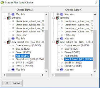
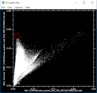
Figure 2.

Figure 3.
* We used this scatter plot just for vegetation because, we know that NIR, RED bands are good for vegetation and NDVI is typically for vegetation.*
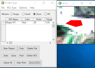
Figure 4.

Figure 5.
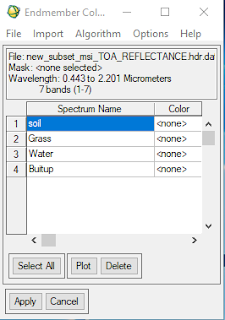
Figure 6.

Figure 7.
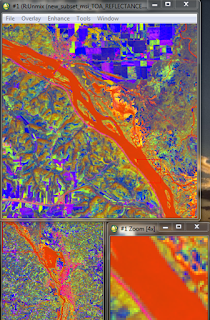
Figure 8.
You can also see the accuracy with in the fractional cover image by using RMS value. We use RMS band with grey window and see which area is the high/low accuracy. High value means high error, therefore in our lab, built-up and bare soil pixels have a high error which is represented as white color in the figure below(Figure 9.).

Figure 9.
Spectral Mixture Analysis
Introduction:
Something we have learn previously such as object based image analysis, we classified as a one single feature. In this lab we are going to further in to that. Many of the images from satellites, we can visually identify land cover/use based on our primary human perception. However, it is not always right, for example, the area that you might think is vegetation may not be just purely vegetation. There should be some other land types that have been mixed with vegetation, such as different types of soil. To distinguish the proportion of land types in certain area, we are required to get endmember which is "pure spectra". In this lab, we are going to use two ways to get endmembers; by 2D scatter plot, and ROI. after that, we can use those endmembers to execute the linear spectral unmixing. After executing unmixing, we are able to distinguish the proportion of the pixel type based on our endmembers. keyword:
Endmember : Endmeember is called "pure" pixel. High spatial resolution imagery is not always good to find the endmember because of intimate mixture. There is variability in nature such as rainfall, soil minerals and growing cycle phase that can impact the spectral profile. Endmember from same features may generate little different spectral profile. Additionally, shadow can be obstacle to make an endmember.Data :
- Landsat8 imagery
- Spatial resolution : 30m
- Bands:
- Coastal Blue
- Blue
- Green
- Red
- NIR
- SWIR 1
- SWIR 2
- Panchromatic
- Cirrus
- TIRS 1
- TIRS 2
- Area / date: La Crosse County, WI / 10/17/2015
Method :
- Load the ENVI and import the image 'new_subset_msi_TOA_REFLECTANCE'
- Go to the 2d scatter plot band choice
- set the Red band as X and NIR as Y

Figure 1.
- Digitize the most vegetated area which is left and top section.
- Get a mean spectral plot then export as a spectral library.

Figure 2.

Figure 3.
* We used this scatter plot just for vegetation because, we know that NIR, RED bands are good for vegetation and NDVI is typically for vegetation.*
- Now we are going to use ROI for rests of endmenbers
- To find pure pixel, first, we need to use enhance tool(Gaussian or Equalization) to see which part of pixel is appropriate to use. (In this case, we use built up area, which is most whitish pixel.)
- Open the ROI tool and find the best fit place that you are going to digitize

Figure 4.
- Save ROI
- Open Spectral Library Builder
- Import the ROI and plot it then save the spectral profile as an endmember.
- Repeat the same process to water and bare soil.
- Once you got all 4 endmembers, stack them all and make a spectral library plot for 4 endmembers afterthat, you are ready to use 'Linear Spectral Unmixing'

Figure 5.
- Select the 'new_subset_msi_TOA_REFLECTANCE' as input
- load up all 4 endmembers
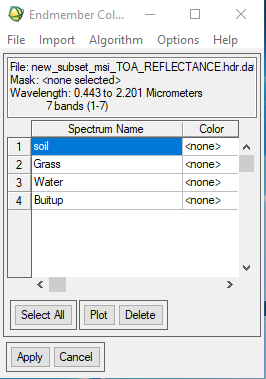
Figure 6.
- Select "apply"
- Load fractional cover bands in ENVI

Figure 7.
Discussion:
Once we got fractional cover image, we are able to distinguish which land cover has the dominant value. The high value indicates the more dominant cover type. For example, if you want to know the component of particular pixel, and you click the center of the Mississippi river, you might get HIGH value on water(value:1.0) additionally, you might get negative value somewhere which means zero existence. Negative, it doesn’t make a sense but it works in linear algebra. We normally count negative as 0 and the reason it shows negative is there should be other place has been overestimated. The overall value should be added up to 1. If the band with over value 1, the amount of its overestimate will be matched with amount of negative value in different band.
Figure 8.
You can also see the accuracy with in the fractional cover image by using RMS value. We use RMS band with grey window and see which area is the high/low accuracy. High value means high error, therefore in our lab, built-up and bare soil pixels have a high error which is represented as white color in the figure below(Figure 9.).

Figure 9.
Comments
Post a Comment